Editor’s note: Today 3/14/15 at some point between 9:26:53 and 9:26:54 it was the most π day of them all. Below is a repost from last year.
Happy π day everybody!
I wanted to write some simple code (included below) to the test parallelization capabilities of my new cluster. So, in honor of π day, I decided to check for evidence that π is a normal number. A normal number is a real number whose infinite sequence of digits has the property that picking any given random m digit pattern is 10−m. For example, using the Poisson approximation, we can predict that the pattern “123456789” should show up between 0 and 3 times in the first billion digits of π (it actually shows up twice, starting at the 523,551,502-th and 773,349,079-th decimal places).
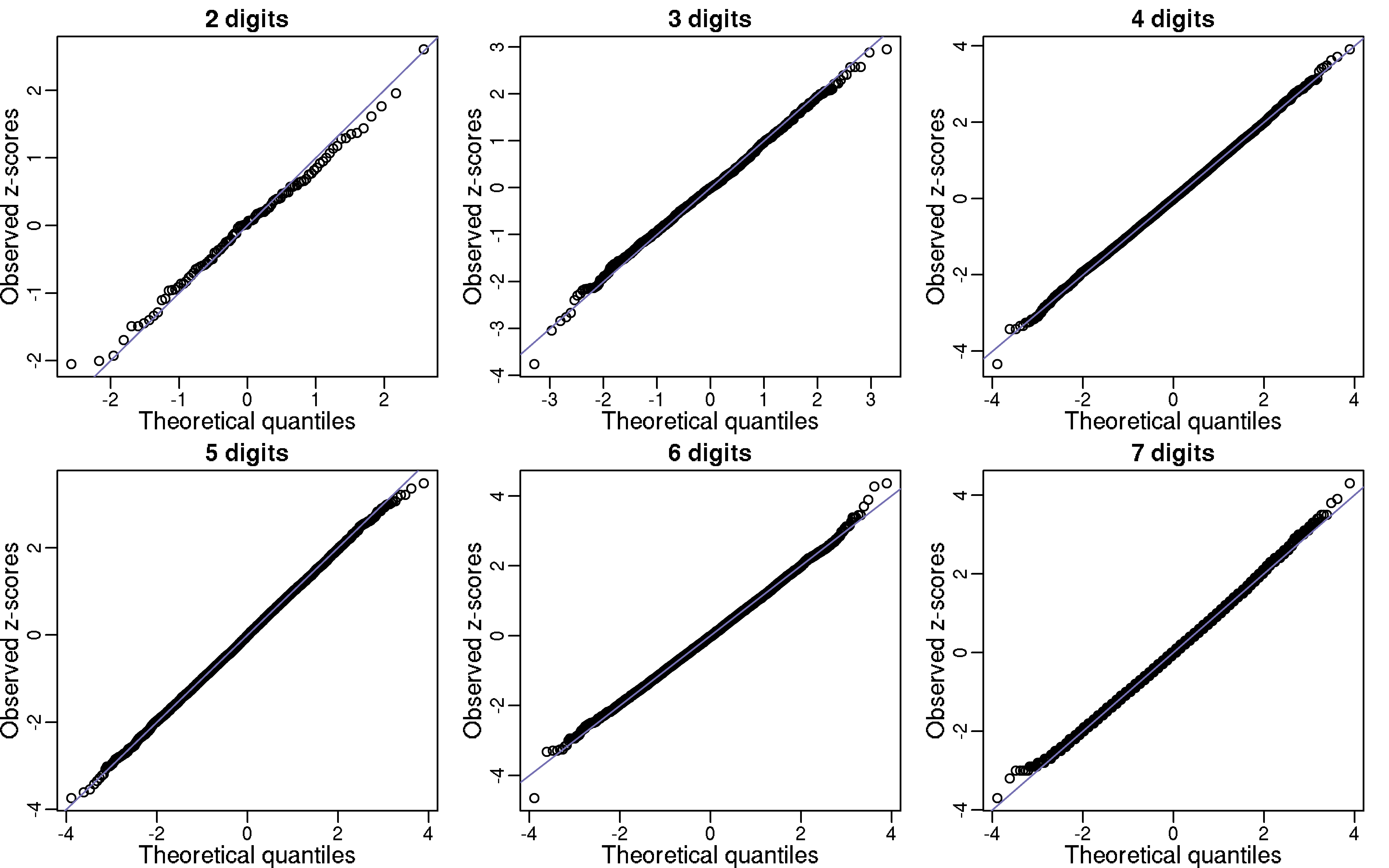
To test our hypothesis, let Y1, …, Y100 be the number of “00”, “01”, …,“99” in the first billion digits of π. If π is in fact normal then the Ys should be approximately IID binomials with N=1 billon and p=0.01. In the qq-plot below I show Z-scores (Y - 10,000,000) / √9,900,000) which appear to follow a normal distribution as predicted by our hypothesis. Further evidence for π being normal is provided by repeating this experiment for 3,4,5,6, and 7 digit patterns (for 5,6 and 7 I sampled 10,000 patterns). Note that we can perform a chi-square test for the uniform distribution as well. For patterns of size 1,2,3 the p-values were 0.84, 0.89, 0.92, and 0.99.

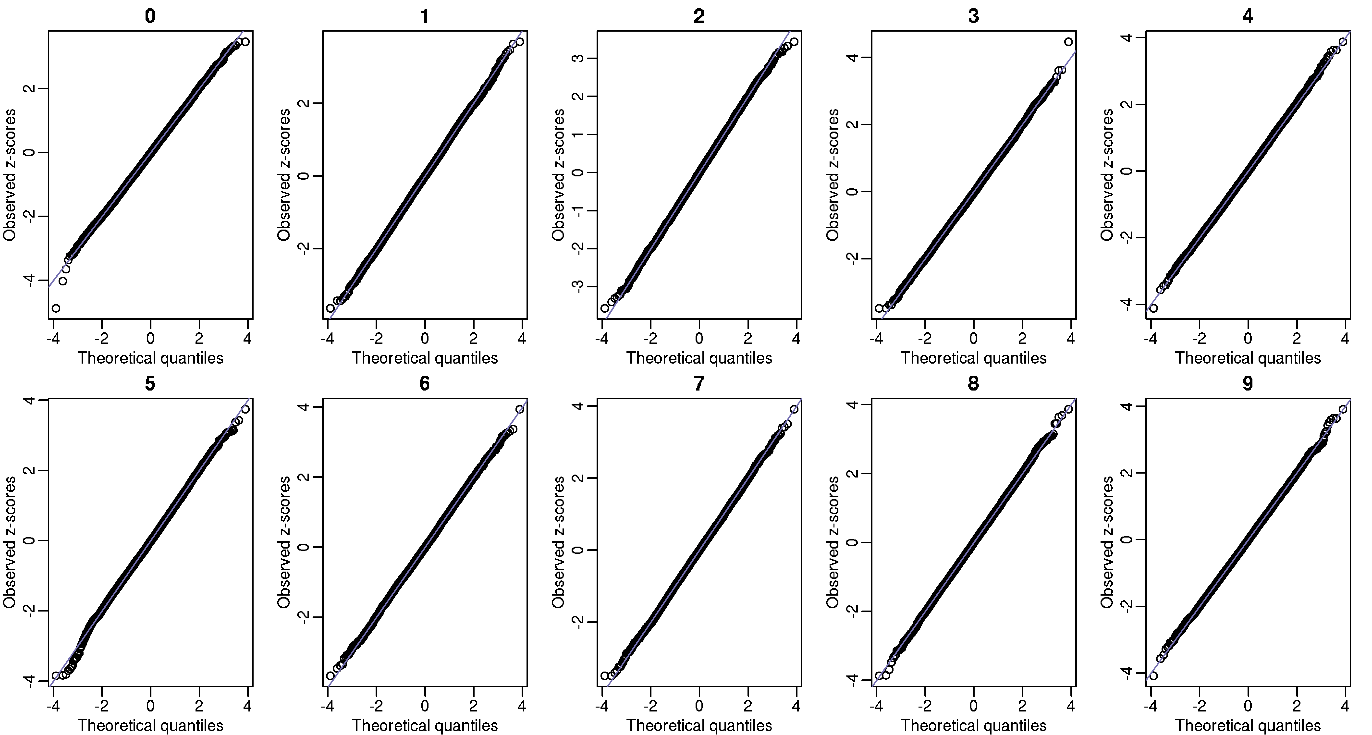
Another test we can perform is to divide the 1 billion digits into 100,000 non-overlapping segments of length 10,000. The vector of counts for any given pattern should also be binomial. Below I also include these qq-plots.

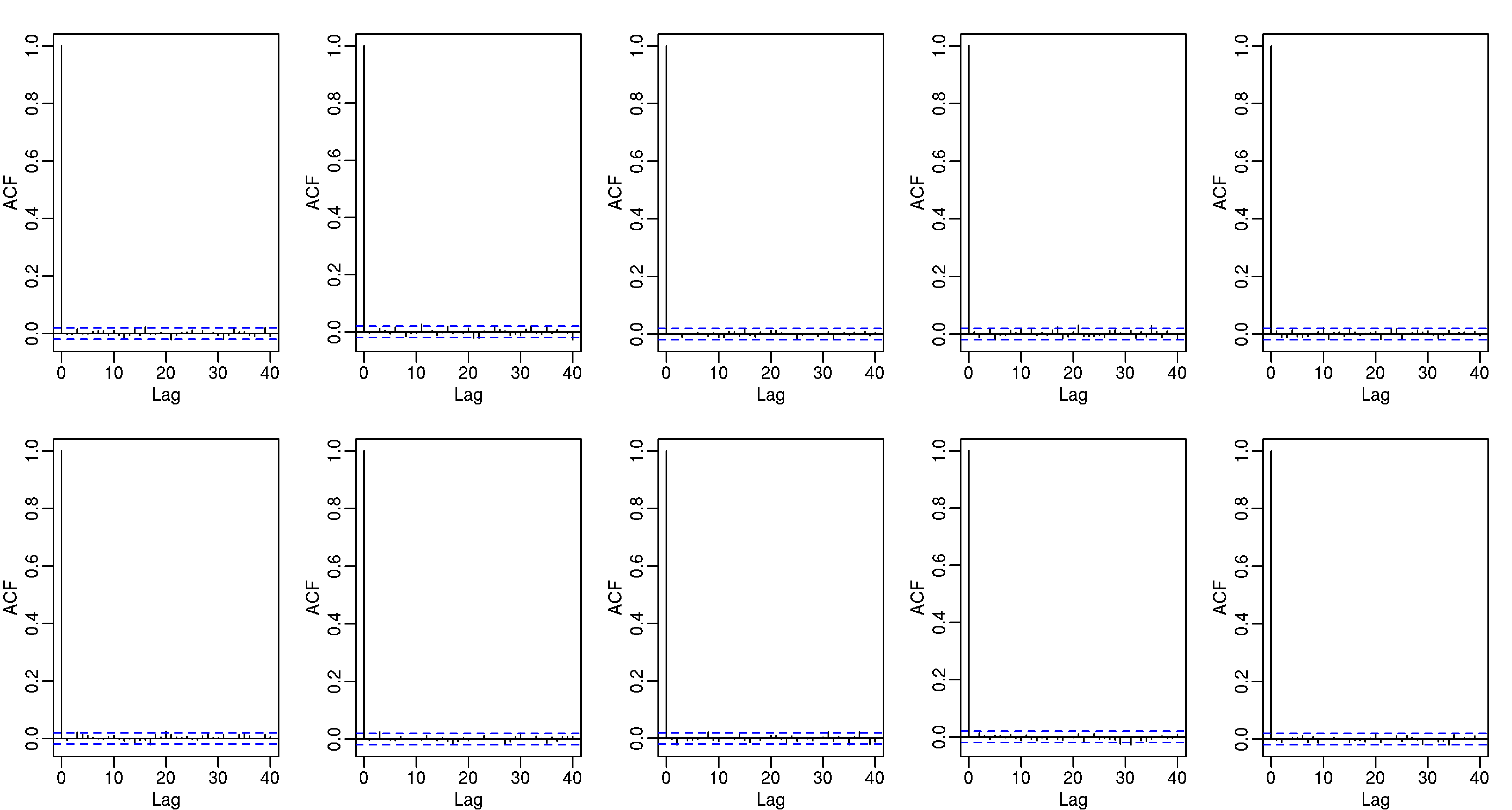
These observed counts should also be independent, and to explore this we can look at autocorrelation plots:

To do this in about an hour and with just a few lines of code (included below), I used the Bioconductor Biostrings package to match strings and the foreach function to parallelize.
library(Biostrings)
library(doParallel)

registerDoParallel(cores = 48)

x <- scan("pi-billion.txt", what="c")
x <- substr(x, 3, nchar(x)) ##remove 3.

x <- BString(x)
n <- length(x)
p <- 1/(10^d)

par(mfrow=c(2,3))
for(d in 2:4){
  if(d<5){
    patterns <- sprintf(paste0("%0", d, "d"), seq(0, 10^d - 1))
    }
  else{
    patterns <- sprintf(paste0("%0", d, "d"), sample(10^d, 10^4) - 1)
  }

  res <- foreach(pat=patterns, .combine=c) %dopar% countPattern(pat, x)

  z <- (res - n*p) / sqrt(n*p*(1-p))

  qqnorm(z, xlab="Theoretical quantiles", ylab="Observed z-scores",
         main=paste(d, "digits"))
  abline(0,1)
  if(d<5) print(1-pchisq(sum((res - n*p)^2 / (n*p)), length(res) - 1))
}

## Now count in segments
d <- 1
m <- 10^5
patterns <-sprintf(paste0("%0", d, "d"), seq(0, 10^d - 1))

res <- foreach(pat=patterns, .combine=cbind) %dopar% {
  tmp <- start(matchPattern(pat, x))
  tmp2 <- floor((tmp-1)/m)
  return(tabulate(tmp2+1, nbins=n/m))
}

## qq-plots
par(mfrow=c(2,5))
p <- 1/(10^d)

for(i in 1:ncol(res)){
  z <- (res[,i] - m*p) / sqrt(m*p*(1-p))
  qqnorm(z, xlab="Theoretical quantiles", ylab="Observed z-scores", main=paste(i-1))
  abline(0,1)
}

## ACF plots
par(mfrow=c(2,5))
for(i in 1:ncol(res))
  acf(res[,i])
NB: A normal number has the above stated property in any base. The examples above a for base 10.