For a few years now I have given a guest lecture on time series analysis in our School’s Environmental Epidemiology course. The basic thrust of this lecture is that you should generally ignore what you read about time series modeling, either in papers or in books. The reason is because I find much of the time series literature is not particularly helpful when doing analyses in a biomedical or population health context, which is what I do almost all the time.
Prediction vs. Inference
First, most of the literature on time series models tends to assume that you are interested in doing prediction—forecasting future values in a time series. I almost am never doing this. In my work looking at air pollution and mortality, the goal is never to find the best model that predicts mortality. In particular, if our goal were to predict mortality, we would probably never include air pollution as a predictor. This is because air pollution has an inherently weak association with mortality at the population, whereas things like temperature and other seasonal factors tend to have a much stronger association.
What I am interested in doing is estimating an association between changes in air pollution levels and mortality and making some sort of inference about that association, either to a broader population or to other time periods. The challenges in these types of analyses include estimating weak associations in the presence of many stronger signals and appropriately adjusting for any potential confounding variables that similarly vary over time.
The reason the distinction between prediction and inference is important is that focusing on one vs. the other can lead you to very different model building strategies. Prediction modeling strategies will always want you to include into the model factors that are strongly correlated with the outcome and explain a lot of the outcome’s variation. If you’re trying to do inference and use a prediction modeling strategy, you may make at least two errors:
- You may conclude that your key predictor of interest (e.g. air pollution) is not important because the modeling strategy didn’t deem to include it
- You may omit important potential confounders because they have a weak releationship with the outcome (but maybe have a strong relationship with your key predictor). For example, one class of potential confounders in air pollution studies is other pollutants, which tend to be weakly associated with mortality but may be strongly associated with your pollutant of interest.
Random vs. Fixed
Another area where I feel much time series literature differs from my practice is on the whether to focus on fixed effects or random effects. Most of what you might think of when you think of time series models (i.e. AR models, MA models, GARCH, etc.) focuses on modeling the random part of the model. Often, you end up treating time series data as random because you simply do not have any other data. But the reality is that in many biomedical and public health applications, patterns in time series data can be explained by clearly understood fixed patterns.
For example, take this time series here. It is lower at the beginning and at the end of the series, with higher level sin the middle of the period.
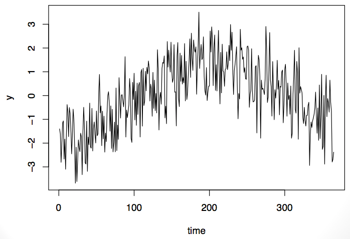
It’s possible that this time series could be modeled with an auto-regressive (AR) model or maybe an auto-regressive moving average (ARMA) model. Or it’s possible that the data are exhibiting a seasonal pattern. It’s impossible to tell from the data whether this is a random formulation of this pattern or whether it’s something you’d expect every time. The problem is that we usually onl have one observation from teh time series. That is, we observe the entire series only once.
Now take a look at this time series. It exhibits some of the same properties as the first series: it’s low at the beginning and end and high in the middle.
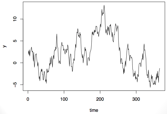
Should we model this as a random process or as a process with a fixed pattern? That ultimately will depend on the what type of data this is and what we know about it. If it’s air pollution data, we might do one thing, but if it’s stock market data, we might do a totally different thing.
If one were to see replicates of the time series, we’d be able to resolve the fixed vs. random question. For example, because I simulated the data above, I can simulate another replicate and see what happens. In the plot below I show two replications from each of the processes.
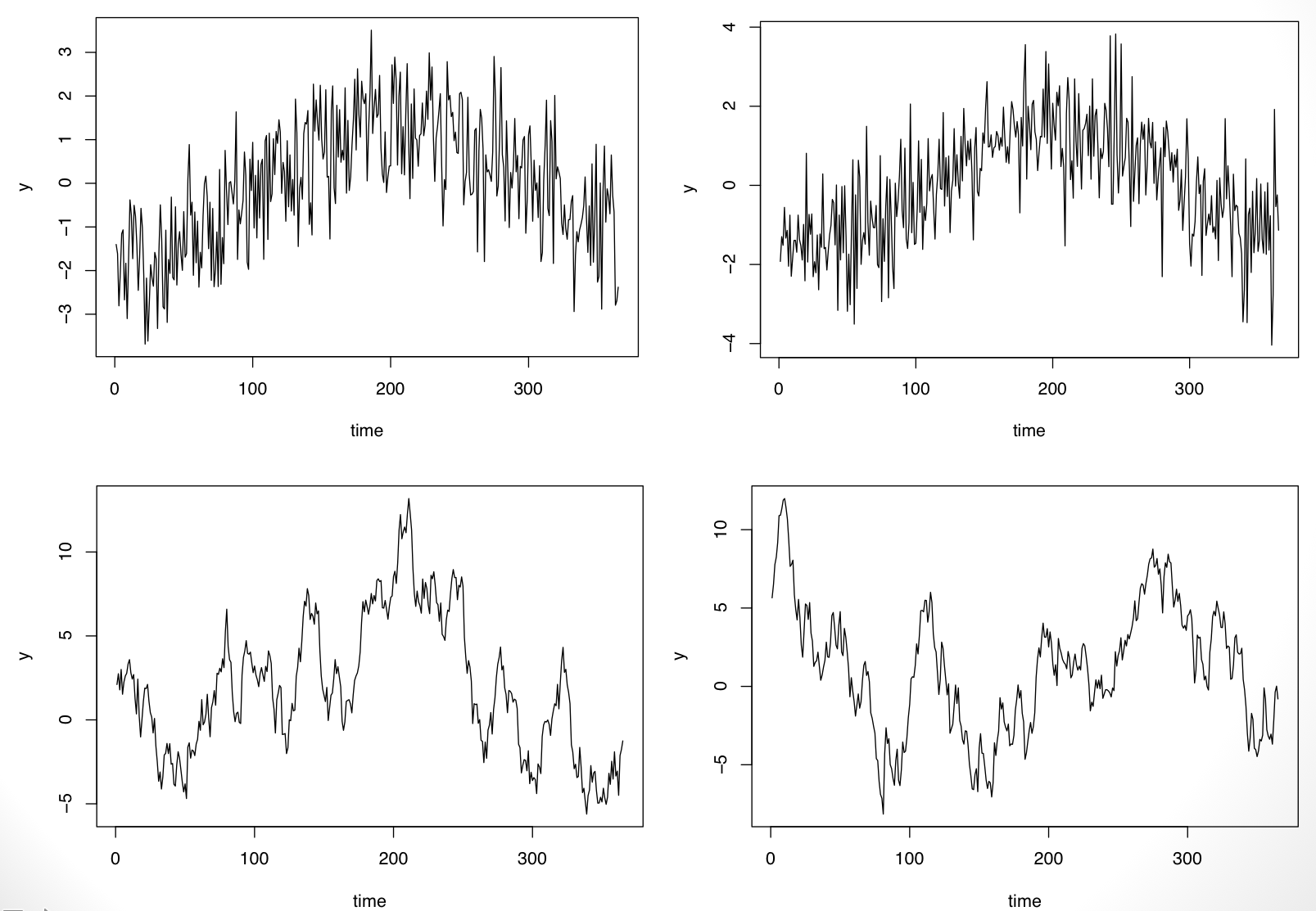
It’s clear now that the time series on the top row has a fixed “seasonal” pattern while the time series on the bottom row is random (in fact it is simulated from an AR(1) model).
The point here is that I think very often we know things about the time series that we’re modeling that we know introduced fixed variation into the data: seasonal patterns, day-of-week effects, and long-term trends. Furthermore, there may be other time-varying covariates that can help predict whatever time series we’re modeling and can be put into the fixed part of the model (a.k.a regression modeling). Ultimately, when many of these fixed components are accounted for, there’s relatively little of interest left in the residuals.
What to Model?
So the question remains: What should I do? The short answer is to try to incorporate everything that you know about the data into the fixed/regression part of the model. Then take a look at the residuals and see if you still care.
Here’s a quick example from my work in air pollution and mortality. The data are all-cause mortality and PM10 pollution from Detroit for the years 1987–2000. The question is whether daily mortaliy is associated with daily changes in ambient PM10 levels. We can try to answer that with a simple linear regression model:
Call:
lm(formula = death ~ pm10, data = ds)

Residuals:
    Min      1Q  Median      3Q     Max
-26.978  -5.559  -0.386   5.109  34.022

Coefficients:
             Estimate Std. Error t value Pr(>|t|)
(Intercept) 46.978826   0.112284 418.394   <2e-16
pm10         0.004885   0.001936   2.523   0.0117

Residual standard error: 8.03 on 5112 degrees of freedom
Multiple R-squared:  0.001244,  Adjusted R-squared:  0.001049
F-statistic: 6.368 on 1 and 5112 DF,  p-value: 0.01165
PM10 appears to be positively associated with mortality, but when we look at the autocorrelation function of the residuals, we see
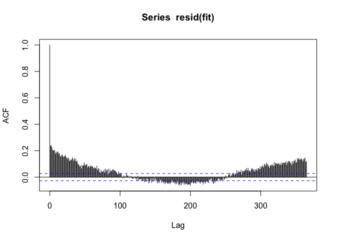
If we see a seasonal-like pattern in the auto-correlation function, then that means there’s a seasonal pattern in the residuals as well. Not good.
But okay, we can just model the seasonal component with an indicator of the season.
Call:
lm(formula = death ~ season + pm10, data = ds)

Residuals:
    Min      1Q  Median      3Q     Max
-25.964  -5.087  -0.242   4.907  33.884

Coefficients:
             Estimate Std. Error t value    Pr(>|t|)
(Intercept) 50.830458   0.215679 235.676     < 2e-16
seasonQ2    -4.864167   0.304838 -15.957     < 2e-16
seasonQ3    -6.764404   0.304346 -22.226     < 2e-16
seasonQ4    -3.712292   0.302859 -12.258     < 2e-16
pm10         0.009478   0.001860   5.097 0.000000358

Residual standard error: 7.649 on 5109 degrees of freedom
Multiple R-squared:  0.09411,   Adjusted R-squared:  0.09341
F-statistic: 132.7 on 4 and 5109 DF,  p-value: < 2.2e-16
Note that the coefficient for PM10, the coefficient of real interest, gets a little bigger when we add the seasonal component.
When we look at the residuals now, we see
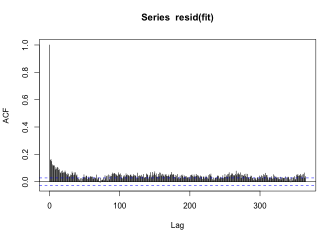
The seasonal pattern is gone, but we see that there’s positive autocorrelation at seemingly long distances (~100s of days). This is usually an indicator that there’s some sort of long-term trend in the data. Since we only care about the day-to-day changes in PM10 and mortality, it would make sense to remove any such long-term trend. I can do that by just including the date as a linear predictor.
Call:
lm(formula = death ~ season + date + pm10, data = ds)

Residuals:
    Min      1Q  Median      3Q     Max
-23.407  -5.073  -0.375   4.718  32.179

Coefficients:
               Estimate  Std. Error t value    Pr(>|t|)
(Intercept) 60.04317325  0.64858433  92.576     < 2e-16
seasonQ2    -4.76600268  0.29841993 -15.971     < 2e-16
seasonQ3    -6.56826695  0.29815323 -22.030     < 2e-16
seasonQ4    -3.42007191  0.29704909 -11.513     < 2e-16
date        -0.00106785  0.00007108 -15.022     < 2e-16
pm10         0.00933871  0.00182009   5.131 0.000000299

Residual standard error: 7.487 on 5108 degrees of freedom
Multiple R-squared:  0.1324,    Adjusted R-squared:  0.1316
F-statistic:   156 on 5 and 5108 DF,  p-value: < 2.2e-16
Now we can look at the autocorrelation function one last time.
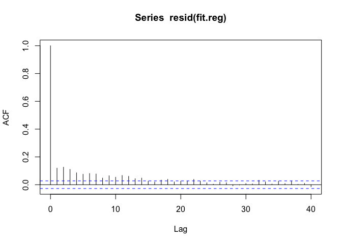
The ACF trails to zero reasonably quickly now, but there’s still some autocorrelation at short lags up to about 15 days or so.
Now we can engage in some traditional time series modeling. We might want to model the residuals with an auto-regressive model over order p. What should p be? We can check by looking at the partial autocorrelation function (PACF).
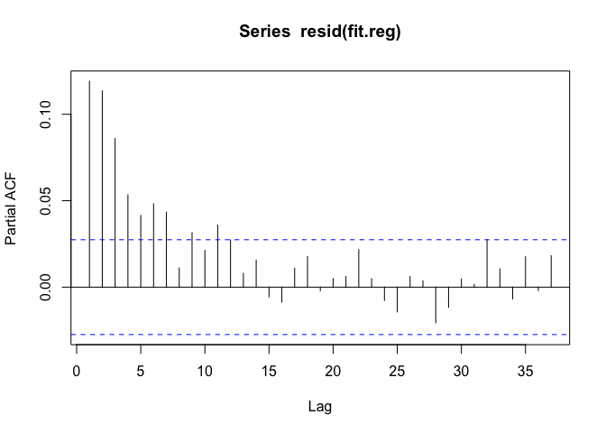
The PACF seems to suggest we should fit an AR(6) or AR(7) model. Let’s use an AR(6) model and see how things look. We can use the arima() function for that.
Call:
arima(x = y, order = c(6, 0, 0), xreg = m, include.mean = FALSE)

Coefficients:
         ar1     ar2     ar3     ar4     ar5     ar6  (Intercept)
      0.0869  0.0933  0.0733  0.0454  0.0377  0.0489      59.8179
s.e.  0.0140  0.0140  0.0141  0.0141  0.0140  0.0140       1.0300
      seasonQ2  seasonQ3  seasonQ4     date    pm10
       -4.4635   -6.2778   -3.2878  -0.0011  0.0096
s.e.    0.4569    0.4624    0.4546   0.0001  0.0018

sigma^2 estimated as 53.69:  log likelihood = -17441.84,  aic = 34909.69
Note that the coefficient for PM10 hasn’t changed much from our initial models. The usual concern with not accounting for residual autocorrelation is that the variance/standard error of the coefficient of interest will be affected. In this case, there does not appear to be much of a difference between using the AR(6) to account for the residual autocorrelation and ignoring it altogether. Here’s a comparison of the standard errors for each coefficient.
               Naive AR model
(Intercept) 0.648584 1.030007
seasonQ2    0.298420 0.456883
seasonQ3    0.298153 0.462371
seasonQ4    0.297049 0.454624
date        0.000071 0.000114
pm10        0.001820 0.001819
The standard errors for the pm10 variable are almost identical, while the standard errors for the other variables are somewhat bigger in the AR model.
Conclusion
Ultimately, I’ve found that in many biomedical and public health applications, time series modeling is very different from what I read in the textbooks. The key takeaways are:
Make sure you know if you’re doing prediction or inference. Most often you will be doing inference, in which case your modeling strategies will be quite different.
Focus separately on the fixed and random parts of the model. In particular, work with the fixed part of the model first, incorporating as much information as you can that will explain variability in your outcome.
Model the random part appropriately, after incorporating as much as you can into the fixed part of the model. Classical time series models may be of use here, but also simple robust variance estimators may be sufficient.