Data on the Comey Effect

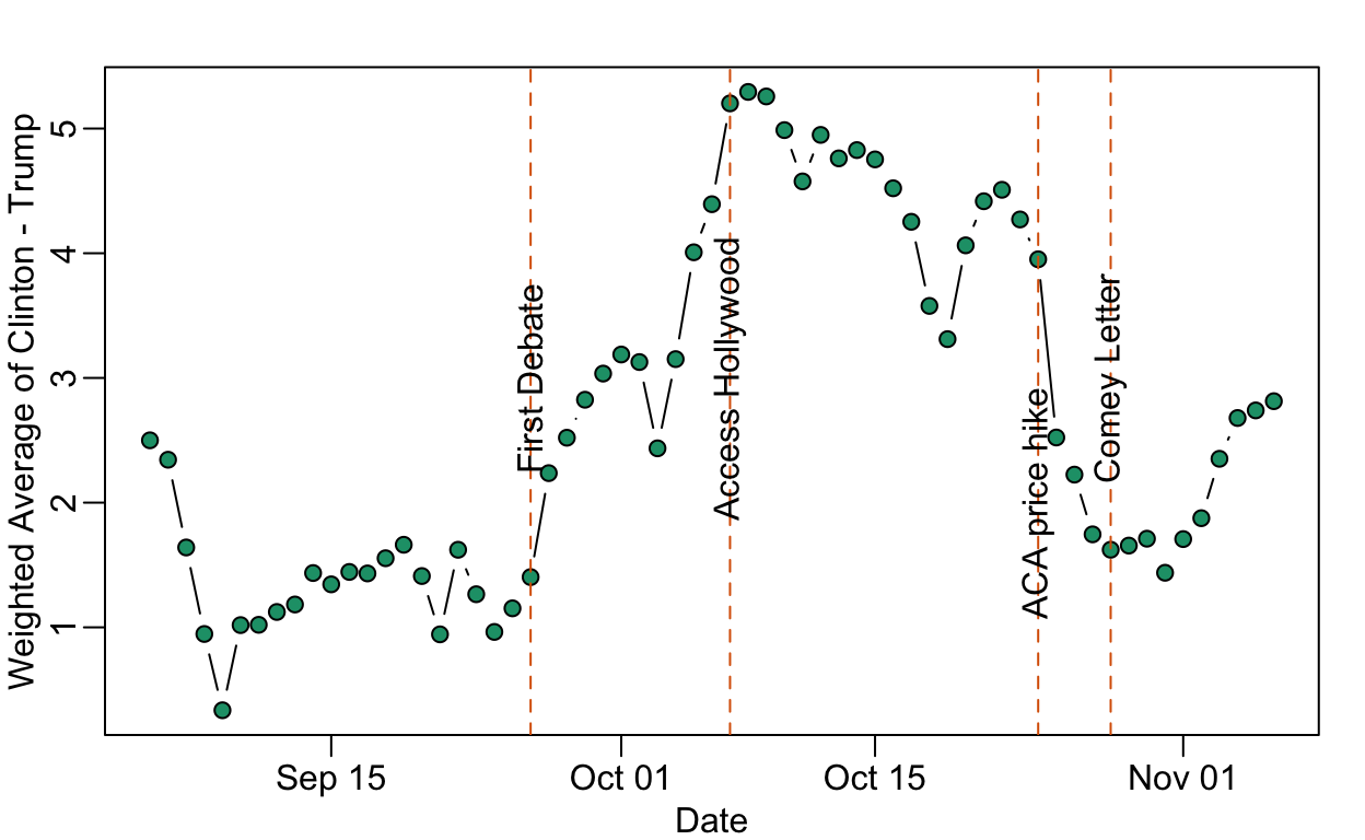
There is currently a debate about whether or not the Comey letter flipped the election. Nate Cohn makes a convincing argument that the letter had little to no effect. Some time ago I looked at this myself and came to a similar conclusion. If anything, it was the ACA price hike announcement that had the bigger effect.

To test out blogdown (thanks Yihui Xie!) I decided to write this post showing the code I used for the simple analysis I performed, hoping to get others to look at the data, point out mistakes, or show me a better way to do what I did. There are many more things I can think of doing, such as account for pollster effect or try to better estimate the day the poll was actually taken.

Here I read-in and wrangle the raw data prepared by 538:

library(tidyverse)
##download data from 538 
url <- "http://projects.fivethirtyeight.com/general-model/president_general_polls_2016.csv"
election_2016 <- read_csv(url)
election_2016 <- filter(election_2016, type=="polls-only")
election_2016$diff <- with(election_2016, rawpoll_clinton-rawpoll_trump) ##define the difference
election_2016$startdate <- as.Date(election_2016$startdate,"%m/%d/%Y") ##turn enddate into date
election_2016$enddate <- as.Date(election_2016$enddate,"%m/%d/%Y") 
start_day <- as.Date("2016-09-01")
election_day <- as.Date("2016-11-08")
dat <- filter(election_2016, startdate > start_day & state=="U.S.") ##after start date and national polls

Then I create a new data frame in which each day for each poll generates a row. I keep track of the reported difference, the number of days in the polling period, and the sample size.

polls <- lapply(1:nrow(dat), function(i){
  days <- (election_day - dat$startdate[i]):(election_day - dat$enddate[i])
  return(cbind( dat[i,c("pollster", "diff")], days, w=1/length(days), 
                n=dat$samplesize[i]))
})
polls <- Reduce(rbind,polls)

Then I compute a weighted average of the difference for each day. Because we are interested in sharp declines, I perform no smoothing other than that imposed by the fact that poll dates span multiple days. If a day was not included in the poll period that poll had 0 weight for that day. If it was include, then the weight was \(1/\mbox{number of days in poll period}\). For example, if poll 1 ran from October 2-4 and poll 2 ran from Oct 1-7, the October 3 estimate would use weights proportional to 1/3 and 1/7 for polls 1 and 2 respectively. They are proportional because weights are scaled to add to 1 for each day. I filtered out days with wieghts less than 10 days. The sample size was not used to compute the weight.

res <- polls %>% 
  group_by(days) %>% 
  filter(sum(w)>3) %>% 
  summarize(avg = sum(diff*w)/sum(w)) %>%
  mutate(date = election_day - days) %>% 
  arrange(date) 

Here is the plot of these weighted averages:

rafalib::mypar()
with(res, plot(date, avg, type="b", pch = 21, bg = 1, xlab = "Date", ylab = "Weighted Average of Clinton - Trump"))
abline(v =  as.Date("2016-10-28"), col = 2, lty = 2)
text(as.Date("2016-10-28"), 3,  "Comey Letter", srt= 90)
abline(v =  as.Date("2016-10-24"), col = 2, lty = 2)
text(as.Date("2016-10-24"), 2, "ACA price hike", srt = 90)
abline(v =  as.Date("2016-10-07"), col = 2, lty = 2)
text(as.Date("2016-10-07"), 3, "Access Hollywood", srt = 90)
abline(v =  as.Date("2016-09-26"), col = 2, lty = 2)
text(as.Date("2016-09-26"), 3, "First Debate", srt = 90)