A recent publication (pay-walled) by Boyle et al. introducing the concept of an omnigenic model has generated much discussion. It reminded me of a question I’ve had for a while about the way genetics data is analyzed. Before getting into this, I’ll briefly summarize the general issue.
With the completion of the human genome project, human geneticists saw much promise in the possibility of scanning the entire genome for the genes associated with a trait. Inherited diseases were of particular interest. The general idea is to genotype individuals with the disease of interest and a group to serve as controls, then test each genotype for association with disease outcome using, for example, a chi-squared test. These are referred to as genome-wide association studies (GWAS).
Since, thousands of GWAS have been performed and have mostly failed to identify variants that explain observed variation: odds ratios for binary disease outcomes tend to be lower than 1.5. In contrast, odds ratios for eye color are above 20. This has generated much debate and speculation about why. Boyle et al. show data that point to the possibility that most inherited traits are so complex that they may involve cumulative effects of a very large proportion of, or even most, variants, but each with very small effects. If this is the case, it has several implications on how we analyze and interpret GWAS data.
Because current technologies permit millions of variants to be tested, current GWAS apply multiple comparison corrections after obtaining a p-value for each variant. The Bonferroni correction for an error rate of 0.05 is the standard, which implies that a p-value in the order of \(10^{-8}\) is needed to reach genome-wide significance. Because the effect sizes are so small, to obtain genome-wide significance, sample sizes in the thousands are needed. As a result, GWAS tend to be expensive relative to other research projects. Furthermore, the better the high-throughput technologies get, the more tests are run, and as a result smaller p-value are required and larger sample sizes are needed. In some cases, after a first GWAS does not yield any variant reaching significance, more samples are collected to increase power.
This brings me to my question. If we know a trait is inherited, then the current hypothesis testing approach may not be appropriate. In particular, controlling the family-wide error rate at 0.05 is too conservative. Why not require a false discovery rate of 0.05, 0.10 or even 0.25? For a typical GWAS how much would conclusions change if we halved the sample sizes and relaxed the significance threshold?
Lacking access to GWAS data (genotypes are hard to get), to illustrate my point I ran a simulation with several genomic regions having a small effect. I simulated data for 5,000 cases and 5,000 controls. A total of 468 genotypes were tested.
spike <- function(x, A=0.02, mu=0, theta=.015, phi=2000)
  A*log((1 - theta)^(abs(x-mu)/theta) * phi + 1)/log(phi)
chr <- rep( 1:9, round(seq(87, 17, len = 9)))
chr_start <- c(which(!duplicated(chr)), length(chr))
chr_start <- (chr_start[-length(chr_start)] + chr_start[-1])/2
P <- length(chr) ## nunmber of features
loc <- 1:P
centers <- c(0.05,0.25,0.55,.8,0.94)*P
As <- c(0.1,0.1,0.125,0.1,0.05)
tmp <- sapply(seq_along(centers), function(i) spike(loc, mu = centers[i], A=As[i]))
effect <- 1 + rowSums(tmp)
set.seed(1)
baseline_p <- rmutil::rbetabinom(P, 100, 0.25, 100) / 100
N <- 5000
disease <- sapply(effect*baseline_p, function(p) rbinom(N, 1, p = p))
control <- sapply(baseline_p, function(p) rbinom(N, 1, p = p))
X <- rbind(control, disease)
if(any(colMeans(X) ==0 | colMeans(X)==1)) stop("One column with MAF=0")
y <- rep(c(0,1), each=nrow(X)/2)
We can obtain odds ratios and p-values and create a Manhattan plot by simply using this code:
res <- apply(X, 2, function(x){
  tab<-table(x,y)
  c(tab[1,1]*tab[2,2]/(tab[1,2]*tab[2,1]),
    chisq.test(tab)$p.value)
})
rafalib::mypar()
plot(loc, -log10(res[2,]) , pch=16, xaxt="n", xlab="Chromosome", ylab="-log (base 10) p-value", ylim=c(0, -log10(0.05/P)))
axis(1, chr_start, seq_along(chr_start), tick=FALSE)
abline(h=-log10(0.05/P), lty=2)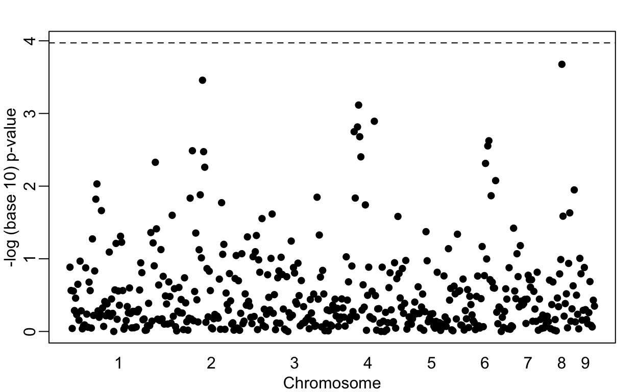
Note that no variant achieves genome-wide significant (dashed line). However, we do see peaks in the plot. If we smooth the odds ratio data, these peaks become even clearer:
logodds <- log(res[1,])
fit <- predict(loess(logodds~loc, span = 0.1), se=TRUE)
mat <- fit$fit + cbind(-2*fit$se.fit,0,2*fit$se.fit)
matplot(loc, mat, type="l", col=c("grey","black","grey"), lty=1, ylim=max(mat)*c(-1,1), ylab="Log odds", xlab="Chromosome", xaxt="n")
axis(1, chr_start, seq_along(chr_start), tick=FALSE)
abline(h=0, lty=2)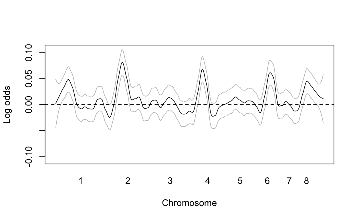
However, in the GWAS world, genome-wide significance at a 0.05 is required. So after obtaining the results above, the next step would be to obtain more funding and double the sample size.
With this larger sample size we now find four regions achieving genome wide significance:
res2 <- apply(X, 2, function(x){
  tab<-table(x,y)
  c(tab[1,1]*tab[2,2] / (tab[1,2]*tab[2,1]),chisq.test(tab)$p.value)
})
plot(loc, -log10(res2[2,]), pch=16, xaxt="n", xlab="Chromosome", ylab="-log (base 10) p-value")
axis(1, chr_start, seq_along(chr_start), tick=FALSE)
abline(h=-log10(0.05/P), lty=2)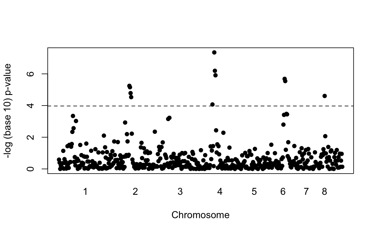
We find four out of the five regions simulated to have effects with no false positives. Here is a plot of the simulated effects:
plot(loc, effect, col=chr, pch=16, xaxt="n", xlab="Chromosome", ylab="Effect")
axis(1, chr_start, seq_along(chr_start), tick=FALSE)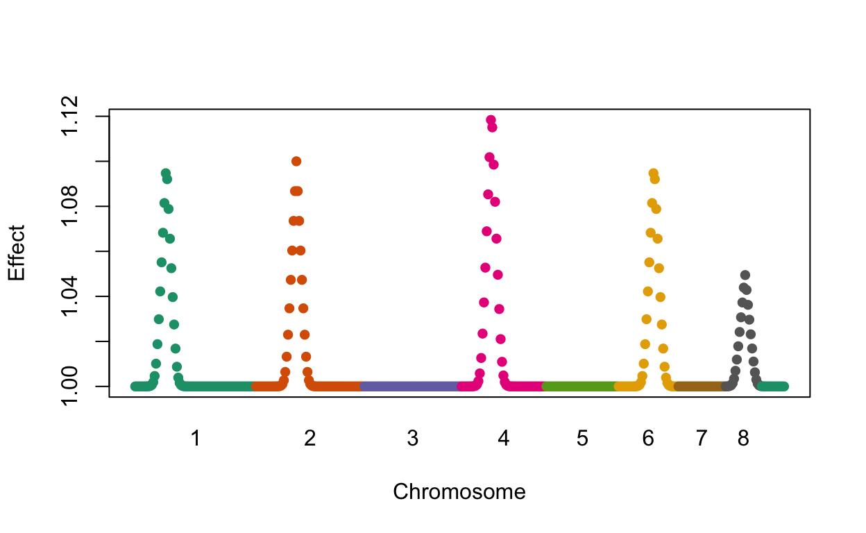
However, note that the shape of the Manhattan plot did not change much with the new data (see figure below). We mostly moved points up by increasing the sample size. But we could have identified those same regions with a relatively low false positive rate, by, for example looking at the top 10 variants, or simply lowering the threshold. In fact, statisticians have beed advocating for other formal statistical approaches.
In the following plot we compare the results using two different sample sizes. We denote the regions simulated to have the strongest effects with black points while the rest are grey.
rafalib::mypar(2,1)
plot(loc, -log10(res2[2,]), col=ifelse(effect>1.01, "black", "grey"), pch=16, xaxt="n",
     xlab="Chromosome", ylab="-log (base 10) p-value", main="Double the sample size")
axis(1, chr_start, seq_along(chr_start), tick=FALSE)
abline(h=-log10(0.05/P), lty=2)
o <- order(res[2,])[1:25] ##top 25 variants
plot(loc, -log10(res[2,]), col=ifelse(effect>1.01, "black", "grey"), pch=16, ylim=c(0, -log10(0.05/P)), xaxt="n", xlab="Chromosome", ylab="-log (base 10) p-value", main="Lower the threshold")
axis(1, chr_start, seq_along(chr_start), tick=FALSE)
abline(h = -log10(max(res[2,o])), lty=2)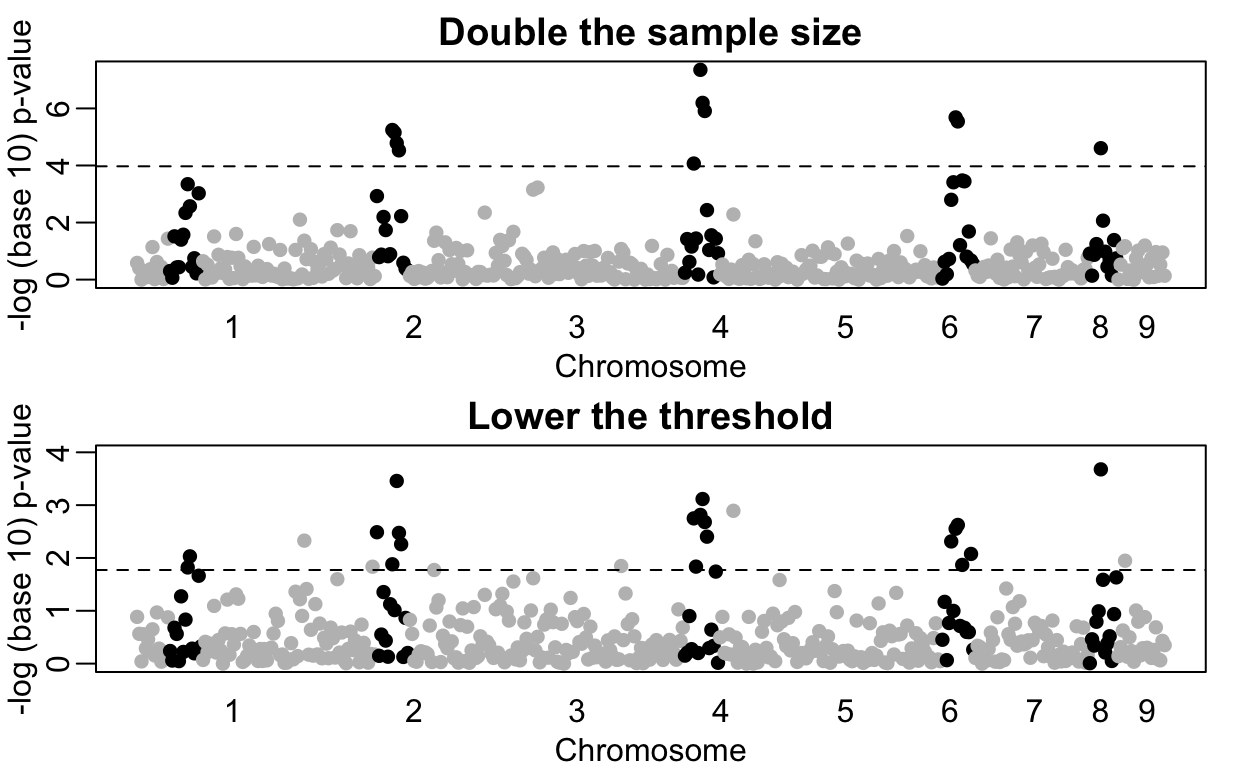
If Boyle et al. are correct, then hypothesis testing is definitely not an appropriate statistical approach for GWAS: we know the null hypothesis is false for most variants. Going forward, to make sense of GWAS data, we should reinvest the millions of dollars currently used to satisfy the Bonferroni correction to measure other endpoints and develop new statistical approaches that can help us understand the molecular cause of disease and improve treatment outcomes.