The NBA season is over and, once again, what I will most remember are King James’ heroics. As a lifelong Boston Celtics fan, I am supposed to hate LeBron James. But I don’t. As a fan of the game of basketball, and a statistician, I just can’t help but be in awe of the best player ever to play the game. Also how can you hate this guy (don’t miss the wrist watch)?

Of all the ridiculous stats one can rattle about LeBron, to me, the most impressive actually relate to a simple one: career totals. The graph below shows you his total points, assists, steals and rebounds as a function of time. The consistency, durability, and all-around production is simply unprecedented. At 33, he is already top 25 all time in three categories: points, assists and steals. If he can keep up his current pace for five more years (I know it’s a big if), he will be top 3 in points, assists and steals, and top 25 in rebounds. No other player comes close.
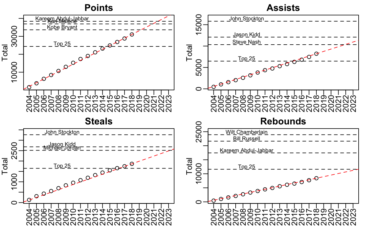
Here is the code that produces the graph above:
library(dplyr)
library(rvest)
url <- "https://web.archive.org/web/20180605212404/https://www.espn.com/nba/player/stats/_/id/1966/lebron-james"
h <- read_html(url)
lebron <-html_nodes(h, "table") %>% .[[3]] %>% rvest::html_table(fill=TRUE) %>% .[,1:17]
names(lebron) <- as.character(lebron[2,])
lebron <-lebron[3:17,]
ind <- 11:17
lebron[ ,ind] <- apply(lebron[,ind], 2, as.numeric)

stats <- c("pts","ast","stl","trb")
full_stats <- c("Points", "Assists", "Steals", "Rebounds")
urls <- paste0("https://web.archive.org/web/20180617065113/https://www.basketball-reference.com/leaders/", stats, "_career.html")
tabs <- lapply(urls, function(url){
  tab <- read_html(url) %>%
    html_nodes("table") %>%
    .[[2]] %>%
    html_table()
   tab <- tab %>% mutate(Player = gsub("\\*", "", Player))
   names(tab)[3] <- "Value"
   tab
})
names(tabs) <- stats
names(lebron)[11] <- "TRB"
ind <- match(toupper(stats), names(lebron))

rafalib::mypar(2,2)
for(i in seq_along(stats)){
  y <- lebron[[ ind[i] ]]
  r <- mean(y)
  x <- 2004:2018

  YLIM <- c(min(y), max(tabs[[i]]$Value))
  YLIM[2] <- YLIM[2]*(1.05)
  XLIM <- c(min(x), 2018 + 5)
  plot(x, cumsum(y), xlim = XLIM, ylim = YLIM, xaxt="n",
       main = full_stats[i], xlab="", ylab="Total")
  axis(side=1, 2004:2023, 2004:2023, las =2)
  abline(-2003*r, r, lty = 2, col = "red")
  j <- c(1:3,25)
  the_names <- tabs[[i]]$Player[j]
  the_names[4] <- paste0("Top 25")
  z <-  tabs[[i]]$Value[j]
  abline(h = z, lty = 2)
  text(2008.5, z, the_names, pos=3, offset = 0.1, cex = 0.7)
}